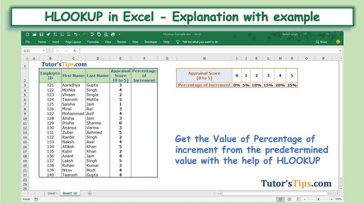
Focus Topic:HLOOKUP in Excel - Explanation with example
Estimated Reading Time:4 mins
Comprehensive academic guide covering core concepts of HLOOKUP in Excel - Explanation with example.
Syllabus-aligned study material with detailed definitions, formats, and practical examples.
Interactive check: Includes a custom practice quiz at the bottom of the article to self-evaluate knowledge.
HLOOKUP in Excel:
In the HLOOKUP Function "H" stand for horizontal and with the help of this formula, we can retrieve the matched value from the selected cells(table array) from up to down means in horizontal order. It supports approximate and exact matched value. It can only look up and retrieve the values in the horizontal order. The lookup value must be in the first row in the selected cells(table array).
Need for HLOOKUP formula: –
With the help of HLOOKUP, we can retrieve the numbers of exact or approximate matched value in the seconds.
It helps in saving time and doing work more efficiently.
it will show the matched value in the column/row where you want. So, we don't need to find the values individually from the selected date and then copy, paste it.
The Feature of HLOOKUP formula: –
It works only up to down. It can only look up the value from the Selected cell(Table_array) from up to the downside. it means from the rows.
This formula provides two types of matched value i.e. approximate and exact.
HLOOKUP always finds the first matched value from the selected cell(Table_array) and retrieve it.
We can use 1 and 0 instead of Ture and False respectively.
It retrieves data based on the Row number.
Explanation of Formula:-
Now, We will explain the Arguments of the formula.
=HLOOKUP(lookup_value, table_array, row_index_num, [range_lookup])
lookup_value: – The lookup value is that value, which will find the exact matched value from the selected cells with this formula. This value is always written in the first row of the selected cells(table array) because HLOOKUP only finds the value in the horizontal order from the selected cells(table array).
table_array: – This is the array of selected cells from which the HLOOKUP will find and retrieve the matched value.
row_index_num: – It means Row Index Number. The number of that row from which we want to retrieve the matched value. The number of rows is counted from the first row of the selected cells(table array).
range_lookup: – It means what type of match you want to show. There is two types of match shown as following: –
Ture: – Approximate Match
False: – Exact Match
If you want to retrieve the Exact match value to show, then write the false and if you approximate matched value, then write true.
Example of Formula: –
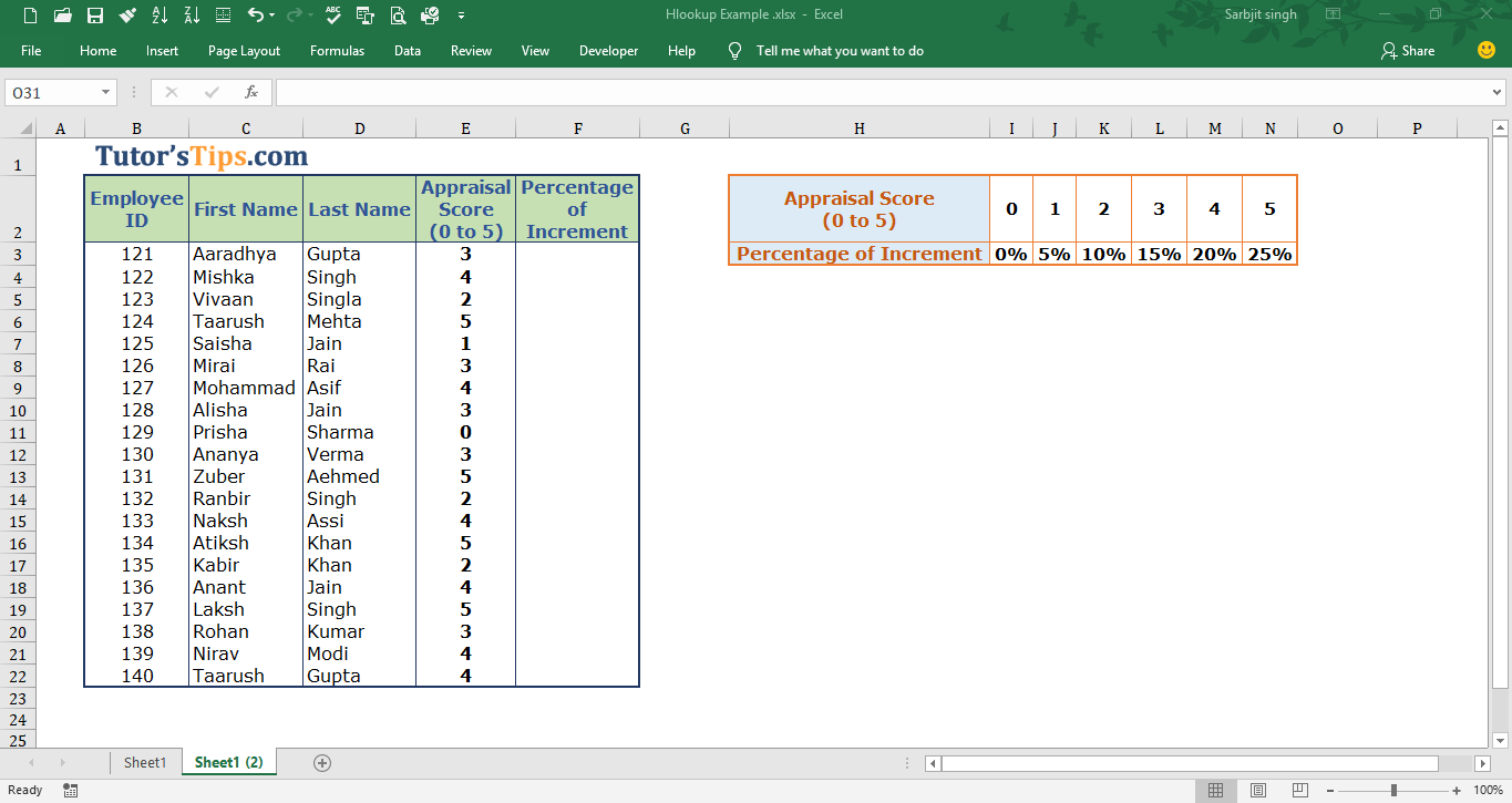
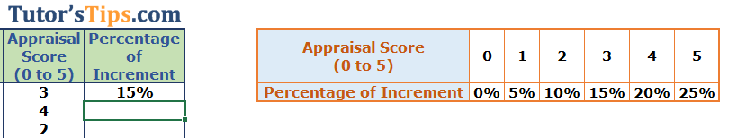
In the following table, we want to retrieve the predetermined percentage of increment from the table according to the appraisal score.
Example of HLOOKUP FormulaSolution:-
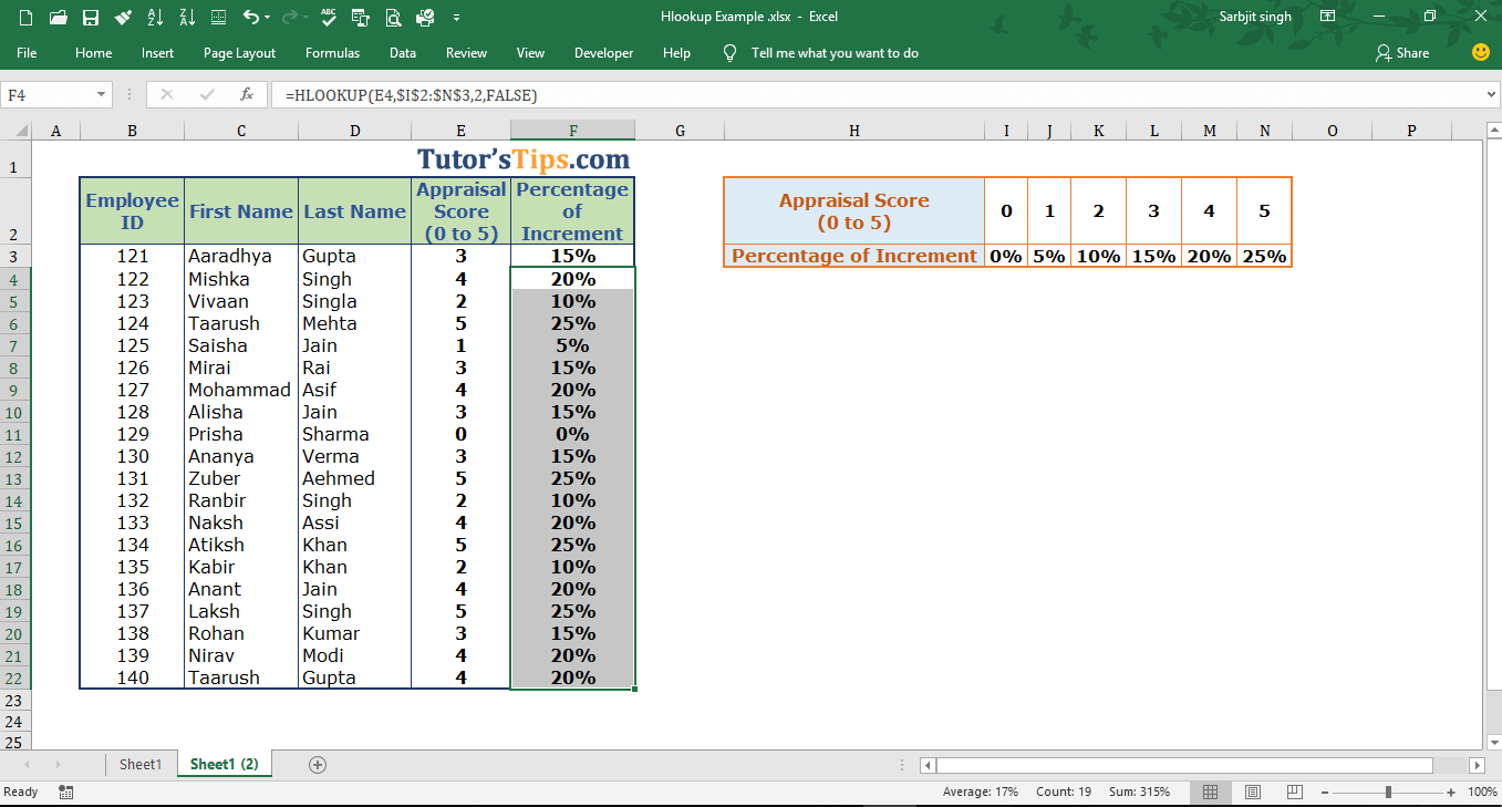
We will use the VLOOKUP formula to retrieve the predetermine the percentage of increment according to the appraisal score.
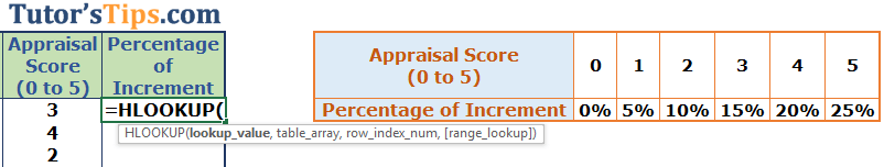
1st Step: –
We will write the “=HLOOKUP( ” in the column of the percentage of increment.
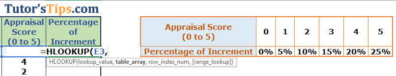
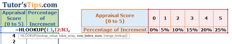
Example of HLOOKUP Formula - Solution Step no. 12nd Step: –
Select the value which we common in both table i.e. Appraisal Score and add a comma at the end.
Example of HLOOKUP Formula - Solution Step no. 23rd Step: –
Select the Table array from which we want to retrieve the value and add a comma at the end.
Example of HLOOKUP Formula - Solution Step no. 34th Step: –
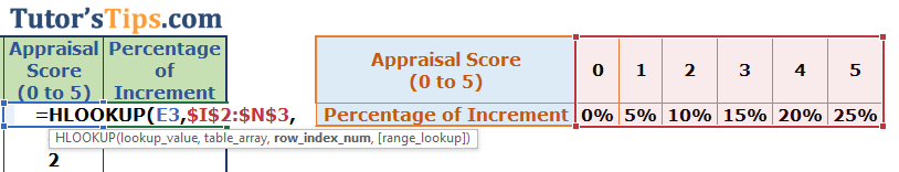
Fix the selection of table array by adding the dollar sign ($) in both the starting and end of the selection like shown below: –
Example of HLOOKUP Formula - Solution Step no. 4This step is needed where we did not want to update the selection of the table array when we copy the whole formula in the remaining cell. 5th Step: –
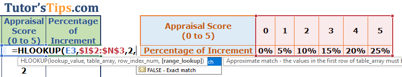
Now select the number of the column of the selected table array of which the value you want to retrieve.
Example of HLOOKUP Formula - Solution Step no. 56th Step:–
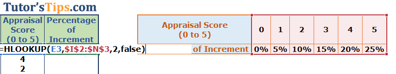
Now choose the mode of matching if you want to match exact value then enter false or 0 or if you want to match approximate value then enter true or 1.
Example of HLOOKUP Formula - Solution Step no. 6Now, press enter key, the formula is complete and you will get the result. Example of HLOOKUP Formula - Solution Step no. 6.1Step No. 7: –
So copy this result(means formula) and then paste it in the remaining cell in which you want to use the same.
Example of HLOOKUP Formula - Solution Step no. 7Thanks Please Share and comment your feedback in the comment box.to buy the Microsoft Excel Click Here.
👤
Author & Educator
Sarbjit SinghB.Com and M.Com
Accounting & Commerce Educator
Sarbjit Singh holds a B.Com and M.Com degree and has over 12 years of teaching experience in double entry bookkeeping, financial accounting, and business studies.
❓ Frequently Asked Questions
What is the main topic of "HLOOKUP in Excel - Explanation with example"?
This guide covers "HLOOKUP in Excel - Explanation with example", focusing on key definitions, step-by-step concepts, applications, and revision guidelines relevant to Excel Formula.
Who can benefit from this guide on "HLOOKUP in Excel - Explanation with example"?
It is primarily curated for Class 11 and Class 12 high school commerce, accounting, and economics students, as well as aspirants preparing for board exams or CA Foundation.
Where can I practice questions related to "HLOOKUP in Excel - Explanation with example"?
You can take our custom-built interactive practice quiz directly on this page to test your understanding of "HLOOKUP in Excel - Explanation with example" instantly.