
Average cost and marginal cost are other constituents of short-run costs with the total cost, fixed cost and variable cost.
Average cost:
The cost of per unit of output is known as Average cost. It can be calculated as:
| AC | = | TC |
| Q |
Here,
AC denotes the average cost
TC denotes the total cost
Q denotes quantity
Illustration:
Suppose the total cost of making 5 units of a commodity is Rs.50. Therefore, the average cost would be calculated as:
| AC | = | 50 |
| 5 |
= 10 units
Thus, the average cost of output can be defined as the cost per unit produced. Also, it can be regarded as the cost of production.
Components :
1. Average Fixed Cost:
It refers to the fixed cost per unit and can be calculated as:
| AFC | = | TFC |
| Q |
Here, AFC denotes Average fixed cost
TFC denotes the total fixed cost
Q denotes the quantity
Representation:
The average fixed cost can be explained with tabular and graphical representation.
Tabular Representation:
The following table shows the average cost with given total costs and units of output produced.
| Output produced(units) | Total Fixed Cost(Rs) | Average Fixed Cost(Rs) |
| 1 | 60 | 60 |
| 2 | 60 | 30 |
| 3 | 60 | 20 |
| 4 | 60 | 15 |
| 5 | 60 | 12 |
The above table shows that when 1 unit is produced, the average fixed cost is Rs.60 and when 5 units of the same commodity are produced, the average fixed cost is Rs.12. In the table, it is cleared that the average fixed cost goes on diminishing with an increase in output.
Graphical Representation:
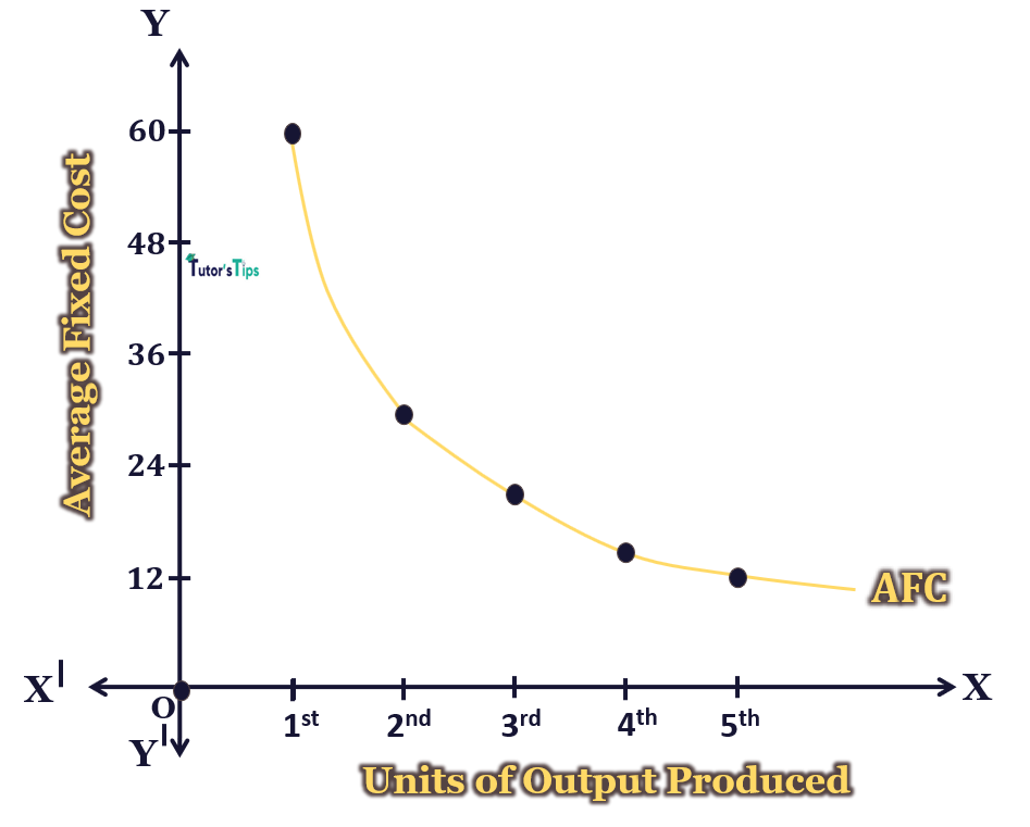
In fig, X-axis shows the output in units and Y-axis shows the average fixed cost. Here, the AFC curve is the average fixed cost curve having a downward slope. Thus, it represents the diminishing AFC with increasing output. Here, It is important to remember that the AFC curve is a rectangular hyperbola which means TFC remains constant at all levels of output.
2. Average Variable Cost:
It refers to the fixed cost per unit and can be calculated as:
| AVC | = | TVC |
| Q |
Here, AVC denotes Average Variable cost
TVC denotes the total variable cost
Q denotes the quantity
Representation:
The average variable cost can be explained with tabular and graphical representation.
Tabular Representation:
The following table shows the average variable cost with given total costs and units of output produced.
| Output produced(units) | Total Variable Cost | Average Variable Cost |
| 0 | 0 | – |
| 1 | 20 | 20 |
| 2 | 36 | 18 |
| 3 | 48 | 16 |
| 4 | 56 | 14 |
| 5 | 60 | 12 |
| 6 | 66 | 11 |
| 7 | 74 | 10.5 |
The above table shows that up to the 5th unit of output, the average variable cost falls but after that, it starts rising. Here, Falling average variable cost represents increasing returns to factor whereas rising average variable cost depicts the decreasing returns to a factor.
Graphical Representation:
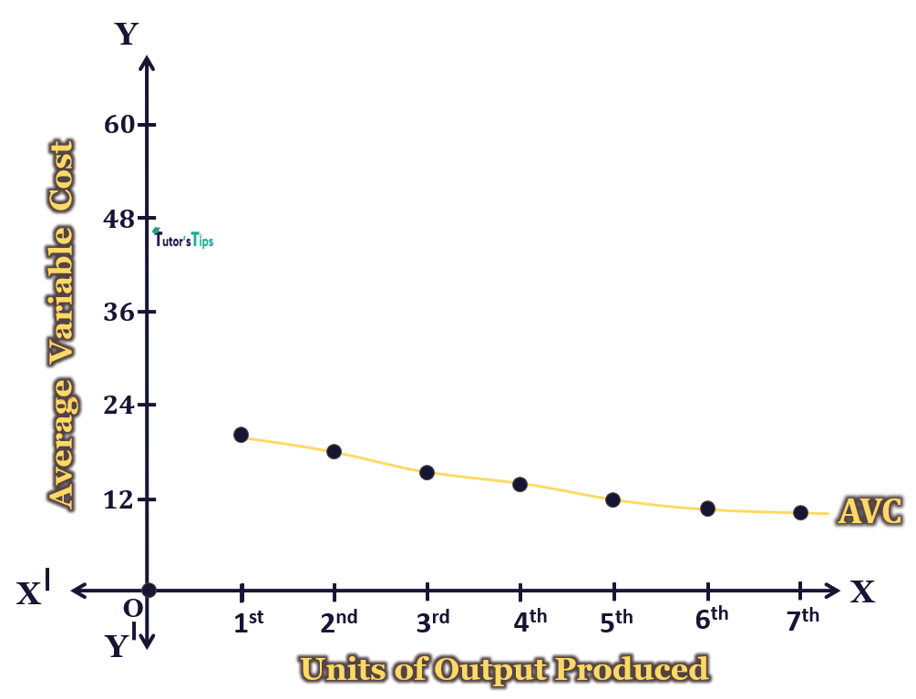
In fig, X-axis shows the output and Y-axis shows the Average variable cost. AVC curve is the average variable cost curve showing that as output increases, the average variable cost tends to fall but after a certain point, it starts to rise. In most of the cases, the AVC is U shaped showing the law of variable proportions. Thus, in initial stages, the AVC tends to fall but later it tends to rise.
3. AC is the summation of AFC and AVC:
AC is the curve showing vertical summation of AFC and AVC curves. It can be understood graphically by aggregating the above table values :
| Output produced(units) | Total Cost | Average Cost |
| 0 | 60 | ∞ |
| 1 | 80 | 80 |
| 2 | 96 | 48 |
| 3 | 108 | 36 |
| 4 | 116 | 29 |
| 5 | 120 | 24 |
| 6 | 138 | 23 |
| 7 | 155 | 22.14 |
The above table shows the average cost of the total cost and quantity given.
Graphical Representation:
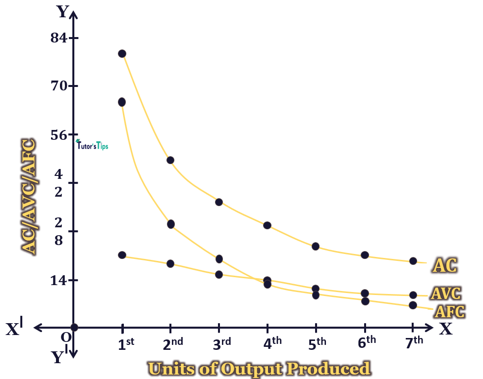
In fig, X-axis shows the output and Y-axis shows the AC, AFC and AVC. It is evident here that in the initial stages, the average fixed cost is more than the average variable cost until these curves intersect each other. But, after that, the AVC is more than AFC. Also, The AC curve is the summation of AFC and AVC. In fig, the AC, AFC and AVC are shown at different levels of output.
Marginal Cost:
It refers to the change in the total cost with the production of an additional unit.
According to Ferguson,
“Marginal cost is the addition to the total cost due to the addition of one more unit of output.”
MCn = TCn – TCn-1
Or
| MC | = | ΔTC |
| ΔQ |
Representation:
The marginal cost can be explained with tabular and graphical representation.
Tabular Representation:
The following table shows the marginal cost with given total costs and units of output produced.
| Output produced(units) | Total Fixed Cost | (TVC)Total Variable Cost | Total Cost | Marginal Cost |
| 0 | 60 | 0 | 60 | – |
| 1 | 60 | 20 | 80 | 20 |
| 2 | 60 | 36 | 96 | 16 |
| 3 | 60 | 48 | 108 | 12 |
| 4 | 60 | 56 | 116 | 8 |
| 5 | 60 | 60 | 120 | 4 |
| 6 | 60 | 66 | 126 | 6 |
| 7 | 60 | 74 | 134 | 8 |
The above table shows that,
MCn = TCn – TCn-1
When 3 units are produced,
MC = TC3 – TC2
= 108-96
= 6
It is evident from the table that the initially MC tends to fall and eventually it tends to rise.
Graphical Representation:
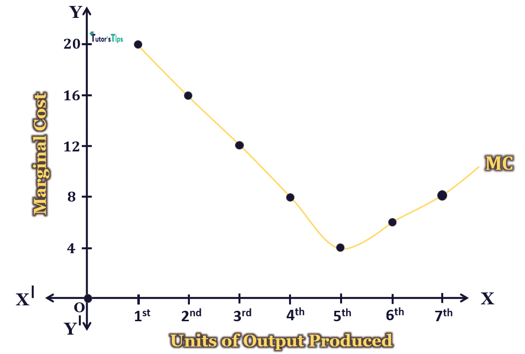
In fig, X-axis shows the output and Y-axis shows the Marginal cost. MC curve is the Marginal cost curve showing that as output increases, the marginal cost tends to fall but after a certain point, it starts to rise. In most of the cases, the MC is U shaped showing the law of variable proportions. Thus, in initial stages, the AVC tends to fall but later it tends to rise.
Thanks, and please share with your friends
Comment if you have any questions.
References:
Introductory Microeconomics – Class 11 – CBSE (2020-21)