The price Consumption curve is the curve made by joining the equilibrium quantities of two commodities at different price levels. Thus, it describes the effect of price on consumer’s equilibrium, assuming other things being the same.
What is Price Consumption Curve:
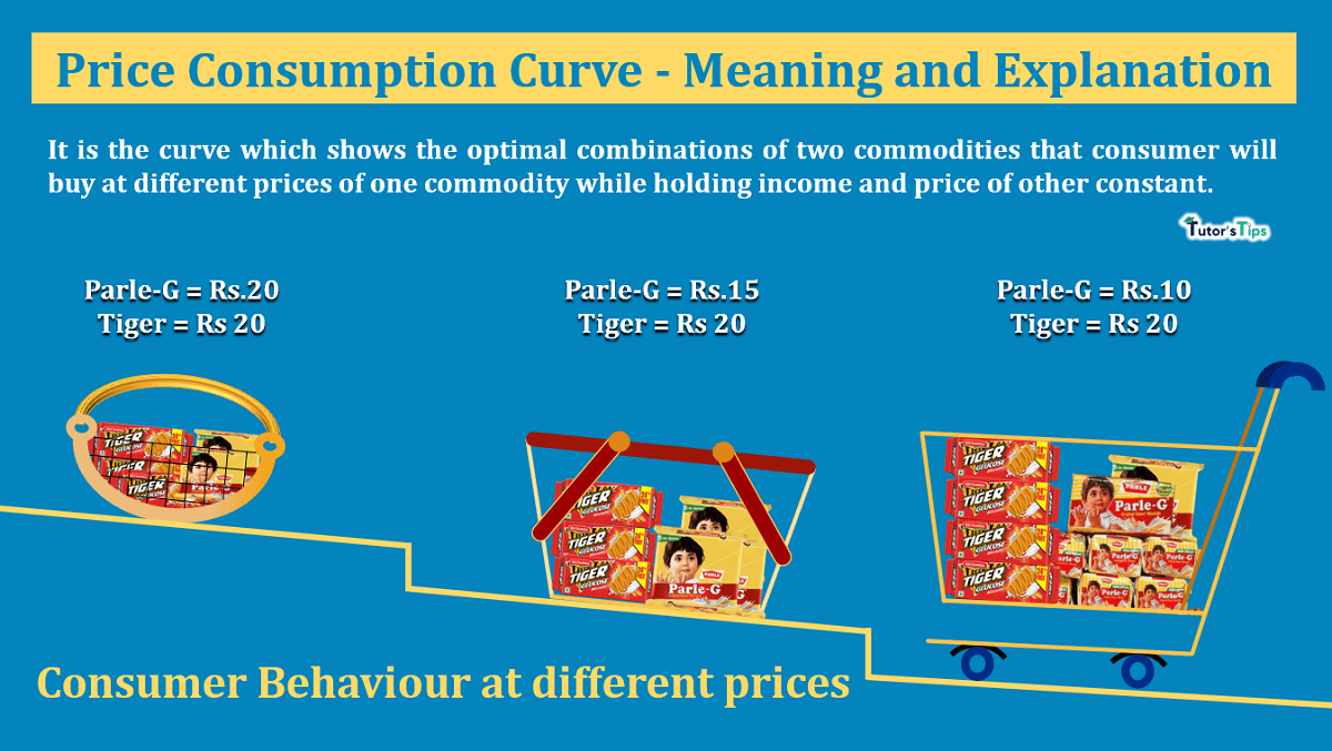
It is the curve which shows the optimal combinations of two commodities that consumer will buy at different prices of one commodity while holding income and price of other constant.
In the words of Ferguson and Maurice,
“The price consumption curve is a locus of equilibrium points relating the quantity of X purchased in relation to its price, money income and all other prices remaining constant.”
When the price of commodity changes, it affects the consumer by making him worse or better than before depending upon the rise or fall in price. In other words, with a fall in the price of a commodity, the consumer’s equilibrium lies at a higher indifference curve and lie on a lower indifference curve with a rise in price. Hence, the line joining the equilibrium points on different budget lines and indifference curves due to change in price is shown by Price Consumption Curve.
Graphical Representation of Price Consumption Curve:
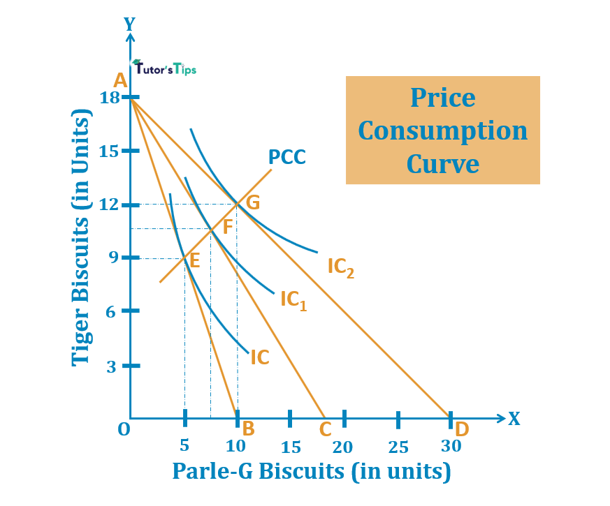
In fig, X-axis shows the quantity of Parle-G Biscuits and Y-axis shows the quantity of Tiger biscuits. The income of the consumer is shown by AB budget line and IC, the original indifference curve shows the maximum satisfaction of the consumer. The consumer is at equilibrium at point E where the budget line AB is tangent to indifference curve IC. It means, that consumer will buy 5 units of Parle-G and 9 units of Tiger biscuits.
Suppose, the price of Parle-G falls to Rs.50, the budget line rotates to right by the proportionate fall in price. The budget line shifts to AC from AB. It will be a tangent to the new indifference curve IC1, at point F. Thus, the new equilibrium point will be F. Now, the consumer will now purchase 7 units of Parle-G and 11 units of Tiger biscuits.
With another reduction in the price of Parle-G to Rs.30, the consumer’s price will shift to AD from AC. As a result, the new budget line will be tangent to the indifference curve IC2 at point G. The consumer will now purchase 10 units of Parle-G and 12 units of Tiger biscuits. The line PCC joining points E, F and G is called the Price Consumption Curve. This curve shows how the consumption of Parle-G biscuits varies with its price varies. Price Consumption Curve shows the quantities of Parle-G, the consumer buys at each price of Parle-G with income and the price of Tiger biscuits held constant.
The Slope of Price Consumption Curve(PCC):
The slope of PCC can be classified as:
- Downward Sloping PCC
- Upward Sloping PCC
- Backward Sloping PCC
- Horizontal Sloping PCC
Downward Sloping PCC :
When the price of commodity changes for which the demand is elastic, the PCC so drawn is downward sloping. It means that a little change in the price of commodity results in more change in the quantity demanded of that commodity.
For Example,
Suppose the price of a commodity-1 falls, it leads to a large increase in the quantity demanded of commodity-1. On the other hand, the quantity demanded of Commodity-2 decreases.
Explanation:
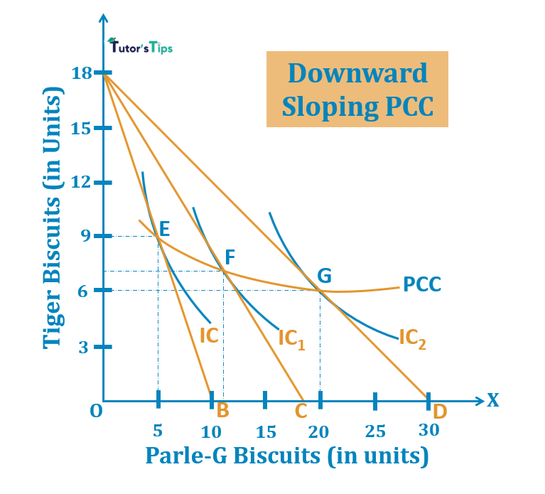
In fig, X-axis shows the quantity of Parle-G Biscuits and Y-axis shows the quantity of Tiger biscuits. AB is the original budget line and IC is the original indifference curve. The consumer is in equilibrium at point E, with maximum satisfaction and available budget of Rs.900. At price being Rs.90 of Parle-G and Rs.50 of Tiger Biscuits, the consumer is consuming 5 units of Parle-G and 9 units of Tiger biscuits at the equilibrium point.
When the price of Parle-G falls to Rs.50, it shifts the budget line to AC and indifference curve to IC1. It also results in the shifting of the equilibrium point from E to F. At point F, the quantity demanded of Parle-G increases to 11 units from 5 units. Also, the quantity demanded of Tiger biscuits decreases to 7 units from 9 units.
Again, when the price reduces to Rs.30, the budget line shifts to AD from AC and indifference curve to IC2 from IC1. It leads to the shifting in equilibrium point from F to G. At new equilibrium point G, the quantity demanded of Parle-G increases to 20 units and that of Tiger biscuits decreases to 6 units from 11 units. Here, the PCC is downward sloping with an increase in the quantity of one commodity and a decrease in the other commodity due to a fall in the price of one commodity.
Here, the Slope of Price Consumption Curve is downward sloping as the demand is elastic. A fall in the price of one commodity increases its demand at a great level whereas reduces the demand for the other commodity to spend available budget with maximum satisfaction.
Upward Sloping PCC :
The slope of the Price consumption Curve generally slopes upward to the right indicating the increase in the purchase of a commodity as the price of that commodity reduces. When the price of commodity changes for which the demand is inelastic, the PCC so drawn is upward sloping. It means, that a change in the price of the commodity affects not only the quantity demanded of that commodity but also, the demand of the other commodity.
For Example,
Suppose the price of a commodity-1 falls, it leads to an increase in the quantities demanded of commodity-1 and commodity-2. It results in upward sloping PCC.
Explanation:
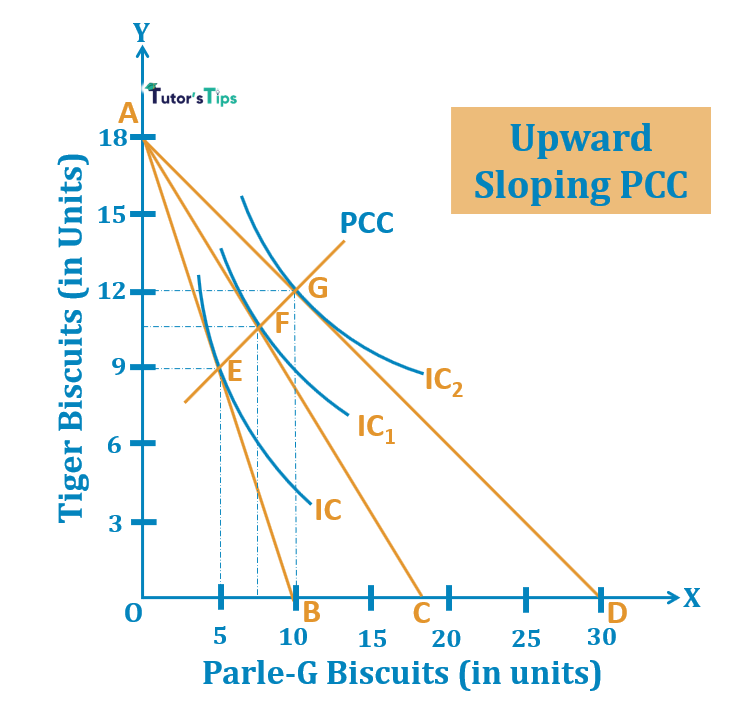
In fig, X-axis shows the quantity of Parle-G Biscuits and Y-axis shows the quantity of Tiger biscuits. Here, AB is the original budget line and IC is the original indifference curve. The consumer is in equilibrium at point E, with maximum satisfaction and available budget of Rs.900. At price being Rs.90 of Parle-G and Rs.50 of Tiger Biscuits, the consumer is consuming 5 units of Parle-G and 9 units of Tiger biscuits at the equilibrium point.
When the price of Parle-G falls to Rs.50, it shifts the budget line to AC and indifference curve to IC1. It results in the shifting of the equilibrium point from E to F. At point F, the quantity demanded of Parle-G increases to 7 units from 5 units. Also, the quantity demanded of Tiger biscuits increases to 11 units from 9 units.
Again, when the price reduces to Rs.30, the budget line shifts to AD from AC and indifference curve to IC2 from IC1. It leads to the shifting in equilibrium point from F to G. At new equilibrium point G, the quantity demanded of Parle-G increases to 10 units and that of Tiger biscuits increases to 12 units from 11 units. Here, the PCC is upward sloping with an increase in both commodities due to a fall in the price of one commodity.
Here, the Slope of Price Consumption Curve is upward sloping as the demand is inelastic. A fall in the price of one commodity increases its demand and quantity demanded of the other commodity to spend available budget with maximum satisfaction.
Backward Sloping PCC :
When the price of a Giffen commodity, the PCC so drawn is backward sloping. It means that a change in the price of the commodity affects not only the quantity demanded of that commodity but also, the demand of the other commodity.
For Example,
Suppose the price of a Giffen commodity-1 falls, it leads to a decrease in the quantity demanded of commodity-1 and increase in quantity demanded of commodity-2. It results in backward sloping PCC.
Explanation:

In fig, X-axis shows the quantity of Giffen commodity-1 and Y-axis shows the quantity of commodity-1. AB is the original budget line and IC is the original indifference curve. The consumer is in equilibrium at point E, with maximum satisfaction and available budget of Rs.900. At price being Rs.75 of Giffen commodity-1 and Rs.50 of commodity-1, the consumer is consuming 10 units of Giffen commodity-1 and 3 units of commodity-1 at the equilibrium point.
When the price of Giffen commodity-1 falls to Rs.50, it shifts the budget line to AC and indifference curve to IC1. It results in the shifting of the equilibrium point from E to F. At point F, the quantity demanded of Giffen commodity-1 decreases to 7 units from 10 units. Also, the quantity demanded of commodity-1 increases to 11 units from 3 units.
Again, when the price reduces to Rs.30, the budget line shifts to AD from AC and indifference curve to IC2 from IC1. It leads to the shifting in equilibrium point from F to G. At new equilibrium point G, the quantity demanded of Giffen commodity-1 decreases to 10 units and that of commodity-1 increases to 15 units from 11 units. Here, the PCC is backwards sloping with the decrease in the quantity of Giffen commodity and an increase in the quantity of the other commodity due to a fall in the price of Giffen commodity.
Here, the Slope of Price Consumption Curve is backward sloping as one of the commodities is Giffen commodity. A fall in the price of that commodity decreases its demand whereas, increases the demand for the other commodity to spend available budget with maximum satisfaction.
Horizontal Sloping PCC :
When the price of commodity changes for which the elasticity of demand is unitary, the PCC so drawn is horizontal sloping. It means that a change in the price of commodity results in a change in the quantity demanded of that commodity only.
For Example,
Suppose the price of a commodity-1 falls, it leads to an increase in the quantities demanded of commodity-1 only and there is no change in the demand of the other commodity. Then, it results in horizontal sloping PCC.
Explanation:

In fig, X-axis shows the quantity of Parle-G Biscuits and Y-axis shows the quantity of Tiger biscuits. AB is the original budget line and IC is the original indifference curve. Here, the consumer is in equilibrium at point E, with maximum satisfaction and available budget of Rs.900. At price being Rs.90 of Parle-G and Rs.50 of Tiger Biscuits, the consumer is consuming 5 units of Parle-G and 9 units of Tiger biscuits at the equilibrium point.
When the price of Parle-G falls to Rs.50, it shifts the budget line to AC and indifference curve to IC1. It results in the shifting of the equilibrium point from E to F. At point F, the quantity demanded of Parle-G increases to 9 units from 5 units and demand for Tiger biscuits remains same at 9 units.
Again, when the price reduces to Rs.30, the budget line shifts to AD from AC and indifference curve to IC2 from IC1. It leads to the shifting in equilibrium point from F to G. At new equilibrium point G, the quantity demanded of Parle-G increases to 15 units and that of Tiger biscuits remain same at 9 units. Here, the PCC is horizontal sloping with an increase in the commodity due to a fall in the price of that commodity and there is no change in the demand for the other commodity.
Here, the Slope of Price Consumption Curve is horizontal sloping as the demand is unitary elastic. A fall in the price of one commodity increases its demand only whereas the demand for the other commodity remains the same for spending available budget with maximum satisfaction.
Thanks Please share with your friends
Comment if you have any question.
References:
Introductory Microeconomics – Class 11 – CBSE (2020-21)

