Derivation of Demand Curve from Price Consumption Curve

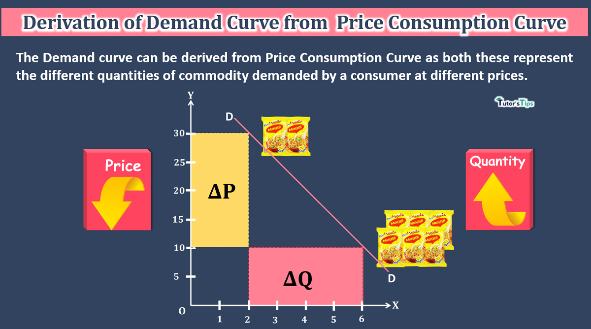
The derivation of the Demand curve from Price Consumption Curve is quite possible as both curves represent the quantity of a commodity demanded at different price levels.

What is the Demand Curve : 

Demand curve indicates the different quantities of the commodity purchased by the consumer at different prices. It also refers to the graphical representation of the relationship between price and quantity demanded.

What is the Price Consumption Curve :

Price Consumption Curve is the curve which shows the optimal combinations of two commodities that consumer will buy at different prices of one commodity while holding income and price of other constant.

In the words of Ferguson and Maurice,

“The price consumption curve is a locus of equilibrium points relating the quantity of X purchased in relation to its price, money income, and all other prices remaining constant.”

When the price of commodity changes, it affects the consumer by making him worse or better than before depending upon the rise or fall in price. In other words, with a fall in the price of a commodity, the consumer’s equilibrium lies at a higher indifference curve and lie on a lower indifference curve with a rise in price. Hence, the line joining the equilibrium points on different budget lines and indifference curves due to change in price is shown by Price Consumption Curve.

Derivation of Demand Curve from Price Consumption Curve:

We can derive the demand curve from the price consumption curve, given the income level of consumer and indifference map. As both these curves represent the relationship between the price of the commodity and its quantity demanded.

The derivation of the demand curve from the price consumption curve includes the substitution as well as the income effect. Therefore, the drawing of the demand curve from PCC is complicated when compared to the demand curve drawn from the demand schedule. 

Assumptions:

1. The money income to be spent on combinations of commodities is constant.
2. The price of one commodity falls.
3. There is no change in the tastes and preferences of the consumer.
4. Price of other commodities remains the same.

In the case of Normal Goods: 

In the case of normal goods, the demand curve so made through the Price Consumption Curve is downward sloping. It defines the negative relationship between price and quantity demanded of a commodity. Thus, for normal goods, the demand increases with a fall in price and decreases with a rise in price.

Graphical Representation:

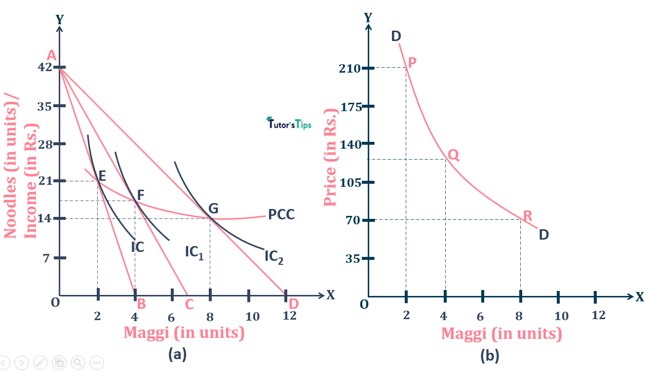
In fig, X-axis shows the quantity of Maggi demanded whereas Y-axis shows the quantity of the other commodity (Noodles) demanded. Here, AB is the original budget line and IC is the original Indifference curve. E is the equilibrium point where budget line AB is tangent to the IC curve. At this point, the consumer is getting maximum satisfaction by spending his income of Rs.840 ( Rs.420 on 2 units of Maggi and Rs.420 on 21 units of Noodles).

Suppose the price of Maggi falls down to Rs.120 from Rs.210. As a result, the budget line shifts to AC and indifference curve to IC₁. Hence, the consumer equilibrium point shifts to F. At this point, the consumer is getting maximum satisfaction by spending Rs.480 on 4 units of Maggi and Rs 360 on 18 units of Noodles. Hence, consumer’s consumption of Maggi increases and quantity demanded of Noodles decreases with a fall in the price of Maggi.

Similarly, When the price of Maggie again, reduced to Rs.70, the budget line and indifference curve shifts to AD and IC₂. As a result, the equilibrium point shifts to F where budget line AD is tangent to indifference curve IC₂. At this point, the consumer is spending Rs560 on 8 units of Maggi and Rs.280 on 14 units of Noodles to get maximum satisfaction.

The curve made by joining these points is the price consumption curve. It indicates that the change in the price of Maggi will bring about change in the equilibrium points of the consumer. Fall in the price of Maggi shifts the quantity demanded from 2 units to 4 units and then to 8 units.

Derivation of the demand curve from Price Consumption Curve:

As it is shown in (a), that at the original budget line AB and indifference curve IC, the quantity demanded of Maggie is 2 units. The Price Consumption Curve shows the different quantities of Maggie purchased by the consumer at different prices. When we plot this price-demand relationship of Maggie is shown on the graph, we get the demand curve.

As shown in Fig (b), If the total income spent by the consumer on Maggie is divided by the number of units consumed, we get the per-unit price of Maggie. It can also be said as the slope of the budget line in (a). we can even draw the demand schedule with this data:

This schedule shows that when the price of Maggie is Rs.210, the quantity demanded is 4 units. In fig(b), It is shown by point P. It implies, the relationship between price and quantity demanded of Maggie. When this price falls to Rs120 and Rs70, the quantity demanded increases to 7 and 12 units respectively, shown by points Q and R. The points P, Q and R in (b) corresponds to E, F and G points in (a). Thus, when we join these points P, Q and R, we get the demand curve DD.

In the case of Giffen Goods: 

In the case of Giffen goods, the demand curve so made through the Price Consumption Curve is upward sloping. It defines the positive relationship between price and quantity demanded of a commodity. Thus, for Giffen goods, the demand increases with a rise in price and decreases with a fall in price.

Graphical Representation:

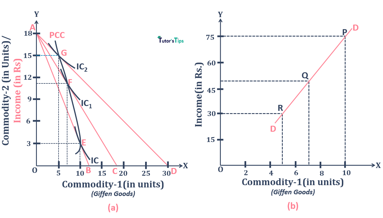
In fig, X-axis shows the quantity of Giffen Commodity-1 demanded whereas Y-axis shows the quantity of the other commodity-2 demanded. Here, AB is the original budget line and IC is the original Indifference curve. And, E is the equilibrium point where budget line AB is tangent to the IC curve. At this point, the consumer is getting maximum satisfaction by spending his income of Rs.900 ( Rs.750 on 10 units of Giffen Commodity-1 and Rs.150 on 3 units of commodity-2 ).

Suppose, the price of Giffen Commodity-1 falls down to Rs.50 from Rs.75. As a result, the budget line shifts to AC and indifference curve to IC₁. And, the consumer equilibrium point shifts to F. At this point, the consumer is getting maximum satisfaction by spending Rs.350 on 7 units of Giffen Commodity-1 and Rs550 on 11 units of commodity-2. Hence, consumer’s consumption of Giffen Commodity-1 decreases and quantity demanded of commodity-2 increases with a fall in the price of Giffen Commodity-1.

Similarly, When the price of Giffen Commodity-1 again, reduced to Rs.30, the budget line and indifference curve shifts to AD and IC₂. As a result, the equilibrium point shifts to F where budget line AD is tangent to indifference curve IC₂. At this point, the consumer is spending Rs150 on 5 units of Giffen Commodity-1 and Rs.750 on 15 units of commodity-2 to get maximum satisfaction.

The curve made by joining these equilibrium points is the price consumption curve. It indicates that the change in the price of Giffen Commodity-1 will bring about change in the equilibrium points of the consumer. Fall in the price of Giffen Commodity-1 shifts the quantity demanded from 10 units to 7 units and then to 5 units.

Derivation of the demand curve from Price Consumption Curve:

As it is shown in (a), that at the original budget line AB and indifference curve IC, the quantity demanded of Giffen Commodity-1 is 2 units. The Price Consumption Curve shows the different quantities of Giffen Commodity-1 purchased by the consumer at different prices. When we plot this price-demand relationship of Giffen Commodity-1 is shown on the graph, we get the demand curve.

As shown in Fig (b), If the total income spent by the consumer on Giffen Commodity-1 is divided by the number of units consumed, we get the per-unit price of Giffen Commodity-1. It can also be said as the slope of the budget lines in (a). we can even draw the demand schedule with this data:

This schedule shows that when the price of Giffen Commodity-1 is Rs.75, the quantity demanded is 10 units. In fig(b), It is shown by point P. It implies, the relationship between price and quantity demanded of Giffen Commodity-1. Suppose, this price falls to Rs50 and then to Rs30, the quantity demanded decreases to 7 and then to 5 units respectively, shown by points Q and R. Here, The points P, Q and R in (b) corresponds to E, F and G points in (a). Thus, by joining these points P, Q and R, we get the demand curve DD. Thus, The upward sloping Demand curve shows the positive relation of price and demand of Giffen Commodities.

Thanks Please share with your friends  

Comment if you have any question.

References:

Introductory Microeconomics – Class 11 – CBSE (2020-21)