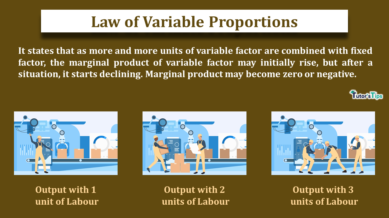
The law of variable proportions explains the effect of overexploitation of factors on output or production.
Meaning of Law of Variable Proportions:
It states that as more and more units of a variable factor are combined with a fixed factor, the marginal product of variable factor may initially rise, but after a situation, it starts declining. Marginal Product may become zero or negative.
In the words of G.Stigler,
“As equal increments of one input are added; the inputs of other productive services being held constant, beyond a certain point the resulting increments of the product will decrease i.e. the marginal products will diminish.”
According to F. Benham,
“As the proportion of one factor in a combination of factors os increased, after a point, first the marginal and then the average product of that factor will diminish.”
For instance, Suppose 4 labours are required to cultivate a hectare of land. The marginal product of labour will increase if initially less than 4 workers are employed. Also, MP would be maximum when 4 workers are employed. Furthermore, it will start declining when more than 4 workers are employed.
Thus, in short, the law of variable proportions indicates the behaviour of output when more and more units of a variable factor are used with a fixed factor.
Assumptions of Law of Variable Proportions:
- There is no improvement or innovation in technology.
- It is based on the possibility of varying proportion in which inputs are combined in production.
- There are some inputs which are kept constant.
Illustration of Law of Variable Proportions:
This law can be explained with the following illustration:
Tabular Representation:
Suppose, using 1 hectare of land as fixed input and labour as a variable factor of input, a producer is able to produce:
| Units of land | Units of labour | Total Product | Marginal Product | |
| 1 | 0 | – | – | Increasing MP implies an increasing return to factor |
| 1 | 1 | 10 | 10-0 = 10 | |
| 1 | 2 | 25 | 25-10= 15 | |
| 1 | 3 | 45 | 45-25= 20 | |
| 1 | 4 | 55 | 55-45= 10 | Diminishing MP implies diminishing returns to a factor including negative returns |
| 1 | 5 | 60 | 60-55 =5 | |
| 1 | 6 | 60 | 60-60= 0 | |
| 1 | 7 | 55 | 55-60 = -5 |
The above table clearly shows that where the MP stops increasing, from that very point it starts diminishing. It represents that as more and more units of labour are used, the MP tends to rise till 3 units of labour are employed. In this situation, TP increases at an increasing rate. Therefore, it is known as the Situation of increasing returns to a factor.
But, with the application of the 4th unit of labour, the situation of diminishing returns set in; MP starts declining and TP increases only at the decreasing rate. After that, the diminishing MP reduces to zero and the total output is maximum when MP is zero. Eventually, MP can be negative. When TP starts declining, the MP becomes negative.
Graphical Representation:


In fig (i), X-axis shows the units of labour used as a variable factor of input and Y-axis shows the total product. And in fig(ii), the X-axis shows the units of labour and Y-axis shows that the marginal product.
The figure depicts :
- MP tends to rise till 3 units of labour are used. This corresponds to point A on the TP and MP curve. This is a situation of increasing returns to a factor.
- When MP is rising, TP tends to rise at an increasing rate. This occurs till point B on the TP as well as MP curve. Therefore, this corresponds to the situation of increasing returns to a factor.
- Beyond 3 units of labour, MP tends to decline and TP increases at a diminishing rate. This occurs between A and B points on TP and MP curve. Therefore, this corresponds to a situation of diminishing returns to a factor.
- When the employment of labour exceeds 6 units, MP becomes negative. Accordingly, TP starts declining. This is a situation of negative returns to factor, occurring beyond point B on TP and MP curve.
Causes of Increasing Returns to a Factor :
Increasing returns to a factor occur because of the following causes:
- Full Utilization of Fixed Factor: In the initial stages, the fixed factor is not fully utilized. The more use of variable factor results in fuller utilization of fixed inputs. Therefore, initially, additional units of labour or variable factor add more and more to total output as long as the fixed factor remain underutilized. Hence, the MP of the variable factor tends to increase.
- Division of labour and increase in Efficiency: Additional application of variable factor enables the process based division of labour. Thus, the specialized workers may be used for different processes which brings efficiency. Accordingly, MP tends to rise.
- Better coordination among factors: As long as the fixed factor remains underutilized, an additional application of variable factor brings better coordination among the factors. As a result, MP increases.
Causes of Diminishing Returns to a Factor :
Increasing returns to a factor occur because of the following causes:
- Fixity of factor: As more and more units of the variable factor are combined with a fixed factor, the latter gets over-utilized. As a result, it suffers wear and tear and loses its efficiency. Hence, it leads to diminishing returns.
- Imperfect Substitute for Factors: Factors of production are imperfect substitutes for each other. The land and labour cannot be used in place of each other. Therefore, the diminishing returns are bound to set in if only the variable factor is increased to increase the output.
- Poor Coordination among factors: Increase in use of one factor affects the ideal ratio of using variable and fixed factor. This results in poor coordination between the factors. Hence, results in diminishing returns.
Thanks, and Please share with your friends
Comment if you have any questions.
References:
Introductory Microeconomics – Class 11 – CBSE (2020-21)


Leave a Reply